This article describes my journey from generating flame fractals using Elixir, to generating a new type of (flame-ish?) fractal in Numerical Elixir. The code is published as a GPL Elixir library at github.com/KeithFrost/frac5.

This summer I’ve been working on personal projects at the Recurse Center (RC). Part of the RC application process involves pitching at least one project that you plan to work on. The frac5 project was inspired by the pitch I wrote for my RC application.

To give due credit, the work I describe here would not exist without Danielle Navarro’s terrific article Art from code V: Iterated function systems (hereinafter referred to as AFC5); I’m going to summarize only those parts of their article which I used for my starting point, but I encourage you to read the whole thing for edification and inspiration.

I had been using Elixir for personal projects for a while, because I find programming with it elegant and fun; I especially enjoy prototyping code using Elixir Livebook running locally. I had read about Numerical Elixir, which extends the language to make it possible to perform the kind of efficient numerical programming often done with NumPy, PyTorch, or similar libraries, but I had not found a use case to motivate learning how to program it myself. I came across AFC5, enjoyed the beautiful images they were able to generate (especially those at the end of the article), and was a little uncomfortable about needing to resort to writing C++ to generate those detailed images quickly. My initial plan was to retrace their steps using only Elixir, and then explore if there was some way to use Numerical Elixir to accelerate the image generation.

Iterated function systems

I will now briefly recap how the beautiful images at the end of AFC5 are generated, although if you want to reproduce all the details from that article precisely, you should of course refer to it, and the code it provides, directly.

Those images are generated by starting with a single point \(p_0\) in a three-dimensional space \({p_0 \equiv (x_0, y_0, z_0)}\). In what follows, we will refer to the coordinates of these points by a second index, so we have \[ p_0 \equiv (p_{0,0}, p_{0,1}, p_{0,2}) \equiv (x_0, y_0, z_0) \]

The point \(p_0\) is then passed through a series of transformations, alternating between linear and non-linear steps, and after each non-linear step, the resulting point is added into the collection of points to be rendered.

In effect, we generate a collection of points \(\{p_k\}, k=0,1,2,...\), where \[ p_{k} = f_k\left( \sum_j A_{k,i,j} \cdot p_{k-1,j} \right). \] The meaning of the linear transformation here should be clear: \[ q_{k,i} = \sum_{j=0}^2 A_{k,i,j} \cdot p_{k-1,j}, i = 0,1,2. \] defines a new 3-D vector \(q_k\) by multiplying the 3-D vector \(p_{k-1}\) by a \(3 \times 3\) matrix \(A_k\). What we mean by \(p_k = f_k(q_{k,i})\) perhaps needs some clarification. The general function \(f_k\) is understood to accept as arguments all three of the components of the 3-D vector \(q_k\), and return all three of the components of the 3-D vector \(p_k\).

In the iterated systems discussed at the end of AFC5, the transformation matrix \(A_k\) at each stage \(k = 1,2,3,...\) is randomly chosen from a set of matrices \(\{M_q\}, q=1,2,...m\), and the function \(f_k(q_k)\) is likewise randomly chosen from a set of non-linear transformations \(\{G_r(q)\}\), defined in AFC5 as \[ \begin{align} G_{0,i}(q) &= q_i + \left( \sum_j q_j^2 \right)^{1/3} \\ G_{1,i}(q) &= \sin(q_i) \\ G_{2,i}(q) &= 2 \cdot \sin(q_i) \end{align} \]

I have taken the liberty here of eliding some manipulations performed in the original AFC5 article, which treat the \(z\) coordinate of the points specially, to ensure that the \(z\) coordinate always remains non-negative, and to average the new \(z\) coordinate \(p_{k,2}\) with its previous value \(p_{k-1,2}\) before finalizing its value. These details might be important if you wish to reproduce the results of that article in detail, but for understanding the extension of that work to follow, it seems best to me to treat all dimensions of the vector space symmetrically, until we are ready to render the pixel data of the image.

Speaking of being ready to render pixel data, we have seen how we can generate an arbitrarily large collection of points \(\{p_k\}, k=0,1,2,...\), but how do we turn those points into an image? In the algorithm described in ACS5, we transform the \((x, y)\) coordinates of the points into indices of a two-dimensional pixel array, and then, if those indices fall within the bounds of the array, set the color of the pixel referenced by those indices to a value determined by some chosen palette for converting \(z\) values to colors.

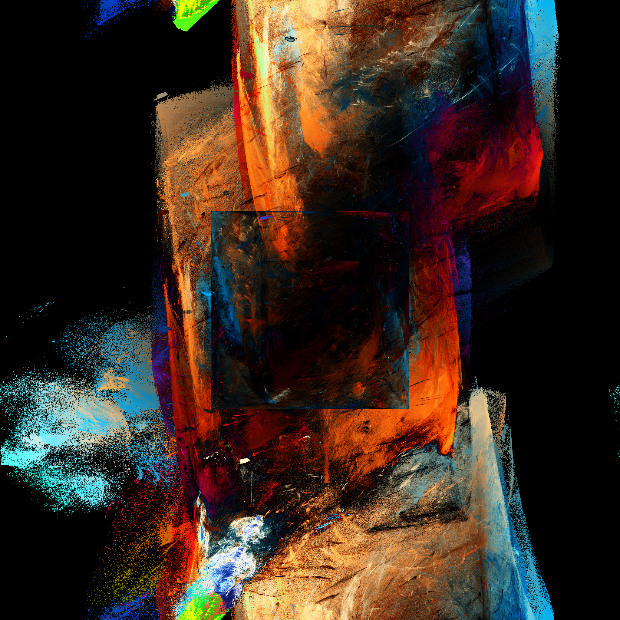
I found I was able to reproduce, as closely as I wished, the work in ACS5, by writing code in ordinary Elixir (without using Numerical Elixir), and it performed well enough to generate some lovely images within acceptable times. For example:

As soon as I was able to generate this image (and several others like it), I became tremendously excited by the potential of the project. I knew that there was much more work I could explore along these lines, by investigating each of the choices that went into creating the images, and finding ways to either optimize the implementation, or expand the range of choices available for artistic purposes. But more than that, I was supremely motivated by the surprising and spectacular beauty of the generated pictures, especially when combined with the stark mathematical simplicity of the means of generating them. To put it bluntly, I was hooked.

Porting to Numerical Elixir

While it is possible to generate interesting and beautiful images using only a few million points using the scheme described in ACS5, more subtle and complex textures become possible by scaling the number of points up to hundreds of millions. And while it is possible to process such large numbers of points on a CPU using a language like Elixir, such “number-crunching” applications are not the forte of the language, and it soon becomes tedious to wait for the image generation process. The author of ACS5 opted to port the algorithm to C++ to achieve better speed; I wanted to find out if it might be possible to do so using the features of Numerical Elixir, especially with a backend programmed to use a GPU.

I quickly realized that there was a significant obstacle to achieving a significant performance improvement of the fractal algorithm presented above using Nx, particularly on the GPU. Many of the performance benefits achieved by libraries like Nx, which manipulate numbers in large, often multi-dimensional arrays, come from being able to compute operations on many elements of these arrays in parallel. This is especially true for the performance enhancements provided by using the GPU. But recall the algorithm presented above, in which we might wish to process hundreds of millions of points \(\{p_k\}, k=0,1,2...\), defined in sequence by some transformation \(p_{k-1} \rightarrow p_k\). If the components of each point \(p_k\) depend on some random choices and the components of the preceding point \(p_{k-1}\), we cannot achieve any high degree of parallelism of the processing of these points, since a processor (either CPU or GPU) cannot process a point until the values from the preceding point (and the random choices) are available.

One means of circumventing this difficulty would seem to be, to replace the single starting point \(p_0\) with an ensemble of starting points, and to achieve the efficiencies of parallelism by collecting ensembles of points processed through the steps of the algorithm in parallel. Unfortunately, my experiments with implementing this approach convinced me that the results did not successfully reproduce the aesthetic features of the beautiful images generated by the original algorithm.

Instead, inspired by another variation on the algorithm I had explored, I decided to try something else. Recall above that there were two distinct random choices made for each transformation of the points: first, a random matrix was chosen for the linear transformation, and second, a random non-linear transformation was chosen. I had already experimented with replacing the random choice of matrix with a simple repeating sequence of matrices. To transform the point \(p_k\), for example, we might use the matrix \(M_{k \bmod m}\), where \(m\) is the number of random matrices initially generated. This gave results which were just as beautiful as the random choice algorithm.

So when I thought about how to make the algorithm more suitable to parallel computation, I was already primed to consider modifying the random choice rule. In particular, I opted to try, instead of randomly choosing one of the non-linear transformations available, to always perform all of the non-linear transformations, and to add all of the points thus generated, both to the set of points used to render the image, and to an ensemble of points to be passed to the next stage of the algorithm. This means that the number of points in the ensemble at each stage of the algorithm grows exponentially with each such application of the non-linear transformations. When the ensemble of points grows sufficiently large, I split it up into batches, in order to avoid having any one block of memory need to be too large. Since blocks of points can be discarded once they are accumulated into the grid used to generate the image pixels, and Elixir allows me to generate a lazy stream of blocks of points for accumulation into the grid, this helps to keep memory usage of the program at any one time under control.

I found removing all of the random choices from the execution of the algorithm in this way both aesthetically and intellectually pleasing. I now had a deterministic algorithm for generating beautiful images, given only a sequence of \(3 \times 3\) matrices, a set of arbitrary (usually non-linear) point transformations to be applied, and a color palette for mapping \(z\) values to colors. Moreover, the algorithm could be made to transform enormous numbers of points in parallel, opening the door to making it possible to accelerate it by running on GPU hardware. But I still wasn’t quite satisfied with the generality of the mathematics. In particular, I wanted to use a wider variety of color palettes than those I had yet defined, and I was uncomfortable with the tedium and what seemed to me the arbitrariness of the choices involved in creating new palettes.

Welcome to the 5th dimension

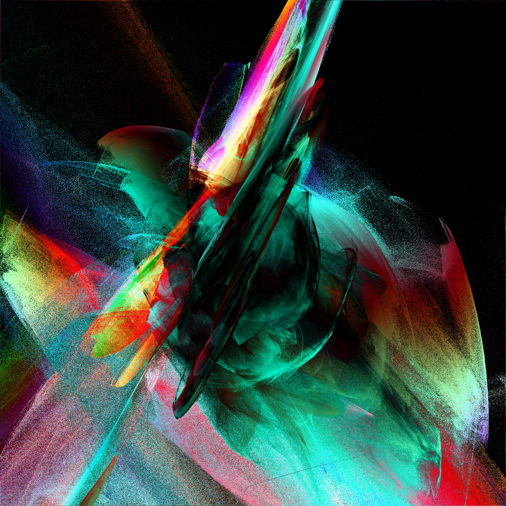
One day I went for a walk, and reflected on how I might remove the need to define a color palette for rendering. After a couple miles of walking, I was struck with an idea. Instead of a three dimensional space \((x,y,z)\), I would process points in a completely analogous way, but in a five dimensional space \((x,y,r,g,b)\). When it came time to render these points to pixel colors, all I would need is a single choice of mapping function from color space coordinate to the corresponding range of pixel values (e.g. \([0,255]\)). Below is the very first image I generated using this new scheme.

It didn’t take very long, after experimenting with generating these 5-D images, that I determined that, in some sense, three degrees of freedom in color space was really a bit more than I wanted to have in most of the final images I was generating. So I modified the rendering algorithm that accumulated the pixel values, so that it accepted the points from the 5-D space, but then subtracted from the color components of each point the portion which was parallel to a chosen (random or arbitrary) unit vector in the 3-D color space, thus flattening the color space to a plane perpendicular to that unit vector.

It was around this time that I got a Mac mini to work with, so I found the EMLX library, which provides an optimized backend for Numerical Elixir which runs on the Mac GPU, and I was quite pleased with the performance boost this gave to the image generation process, allowing me to generate images by processing roughly 300 million points in just a few seconds.

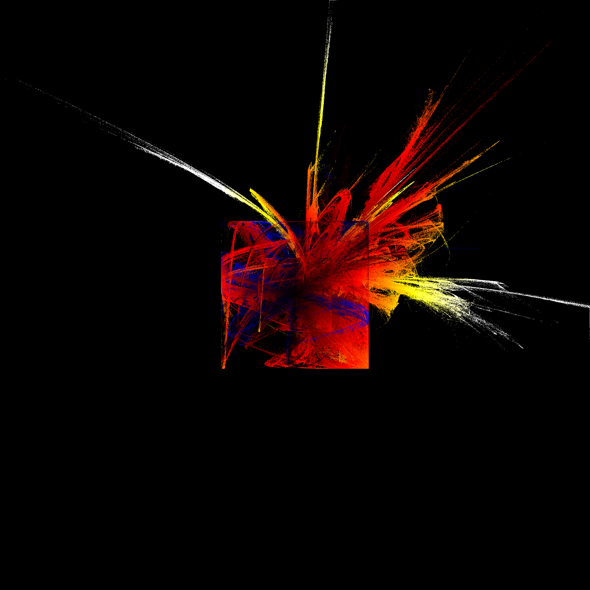
The effects of flattening the color space, and using as many points as I wanted, can be seen in the next sample image.

Themes and variations

If it’s not already clear, I should point out that I experimented freely with as many aspects of the image generation process as I could recognize as choices, to discover if I could produce effects that I found pleasing. When it came time to publish a library of code for this project, it was rather difficult to decide what choices should be hard coded, as opposed to keeping the library as flexible as possible, to support whatever I or other users of the library might want to do with it in the future.

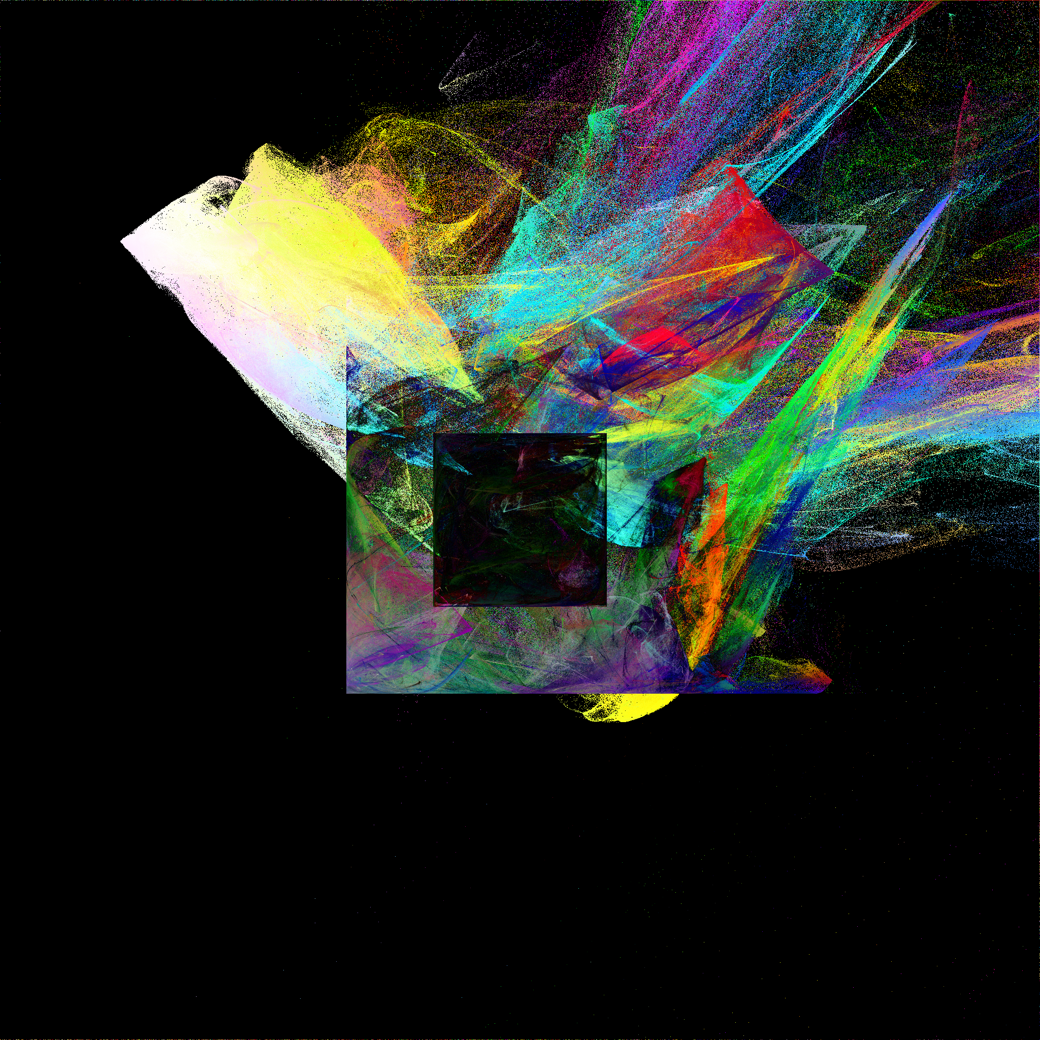
One of the features of the algorithm that I ended up experimenting with, was the choice to select the points right after the non-linear operations, as those to send to the rendering process, as opposed to the points right after the matrix multiplications. By performing the non-linear operations first, and sending points to rendering after the matrix multiplication, the prominent “squares” (projections of 5-D hypercubes) in the earlier images, which were artifacts of the \(C\cdot\sin(q_{k,i})\) non-linear transformations, could be removed, which was a feature I sometimes wanted. I ended up compromising, by writing the algorithm so that it sent the points to rendering after the sequential, usually linear operations, but adding an optional argument to the function which generates the stream of linear operations, which allows the caller to specify some other operations (presumably non-linear) to be interleaved between the linear transformations in the sequence. The image which heads this article, was generated by simply rendering points after each linear transformation.

A walk through the code

The core of the library, as currently implemented, is divided into three major modules: Frac5.Affine, Frac5.Transforms, and Frac5.Pixels. There are two other modules, Frac5.Pnm for reading and writing Netpbm image files, and Frac5.Extract, for computing a zcolor unit vector from an input image, but we will not delve into those two modules here.

Frac5.Affine

defmodule Frac5.Affine do
  import Nx.Defn
  defstruct matrix: nil, txform: nil

  @pi2 2.0 * :math.acos(-1.0)
  @pi4 2.0 * @pi2
  @pi10 5.0 * @pi2

  defn affine_tx(matrix, pts) do
    Nx.remainder(Nx.dot(pts, matrix) + @pi10, @pi4) - @pi2
  end

  def generate(scale) do
    variance = scale * scale

    matrix =
      for _i <- 0..4 do
        for _j <- 0..4 do
          :rand.normal(0.0, variance)
        end
      end
      |> Nx.tensor()

    %Frac5.Affine{matrix: matrix, txform: fn pts ->
      affine_tx(matrix, pts)
    end}
  end

  def generate_stream_init(n, scale, txfms \\ []) do
    affs = Enum.map(1..n, fn _i -> generate(scale) end)

    init_points =
      Enum.flat_map(affs, fn aff -> Nx.to_list(aff.matrix) end)
      |> Nx.tensor()
      |> Nx.multiply(1.0 / scale)

    txforms = interleave(
      Enum.map(affs, fn aff -> aff.txform end),
      txfms)
    stream = Stream.cycle(txforms)
    {stream, init_points}
  end
end

Declaring import Nx.Defn allows us to use the Numerical Elixir numerical function definition

  defn affine_tx(matrix, pts) do
    ...
  end

which is notably not equivalent to a standard Elixir function definition. Instead, this form is meant to declare functions of Numerical Elixir tensor objects, which can be compiled to run on whatever backend is configured. The semantics of operations inside an Nx numerical function are handled differently: for example, notice that we use the + symbol to add a floating point constant to a tensor, which would raise an error if it were attempted in ordinary Elixir code.

You may also note that we define the affine transformation a little differently than the simple formula provided in the earlier discussion. This is because I chose to define the five-dimensional space in which all our operations take place to be a hyper-toroid, with the space wrapping around at fixed boundaries in each dimension. All coordinates are constrained to fall in the range \([-2\pi, 2\pi]\), and any coordinate which would fall outside that range, is reinterpreted modulo \(4\pi\), to fall back inside the range.

The generate_stream_init() function will usually be the main entry point for this module. It creates an infinite (lazy) stream of linear transformations, repeating every n linear steps, possibly interleaved with a likewise repeating list of other transformations supplied by the programmer. It returns this infinite stream, along with a set of initial points, which are constructed by simply taking the rows of the generated matrices.

(Note that interleave is a private function to this module, which does just what the name suggests: accepts two lists as arguments, and generates a list by interleaving available values from each of its two inputs until both inputs are exhausted.)

Frac5.Transforms

defmodule Frac5.Transforms do
  import Nx.Defn

  @pi2 2.0 * :math.acos(-1.0)
  @pi4 2.0 * @pi2
  @pi10 5.0 * @pi2

  defn expand(pts) do
    s2 = Nx.sum(pts * pts, axes: [-1], keep_axes: true)
    Nx.remainder(pts + Nx.pow(s2, 0.25) + @pi10, @pi4) - @pi2
  end

  defn contract(pts) do
    s2 = Nx.sum(pts * pts, axes: [-1], keep_axes: true)
    pts * Nx.pow(s2, -0.33)
  end

  defn wmean(pts) do
    Nx.window_mean(pts, {2, 1}, padding: :same)
  end

  defn sin2(pts) do
    2.0 * Nx.sin(pts)
  end

  def default_parallels() do
    [&expand/1, &contract/1, &Nx.cos/1]
  end

  @chunk_limit 100_000

  def points_stream(txform_stream, init_points, parallels) do
    Stream.transform(txform_stream, [init_points], fn txform, pts_stream ->
      next_stream =
        Stream.flat_map(pts_stream, fn pts ->
          {n, _} = Nx.shape(pts)

          if n >= @chunk_limit do
            Enum.map(parallels, fn par -> txform.(par.(pts)) end)
          else
            ppts =
              Enum.map(parallels, fn par -> par.(pts) end)
              |> Nx.concatenate()

            [txform.(ppts)]
          end
        end)

      {next_stream, next_stream}
    end)
  end
end

Note that the expand function is a bit different than the transformation from AFC5: not only does it apply the wrapping behavior to \([-2\pi,2\pi]\), but the power applied is \(1/4\) instead of \(1/3\). There are many such detailed choices open to one generating these fascinating images: the user of this library can easily supply their own function definitions. There is also a contract function which I found interesting, as well as the wmean, which simply averages every two adjacent points in its input. Twice the sin function still makes an appearance, but the defaults I wrote use cos instead. Again, the point is not to repeat exactly the same image generation techniques, but to experiment and find what is most interesting in the moment.

The main utility function here is points_stream(), which accepts as arguments a stream of transforms, a tensor of initial points, and the (usually non-linear) list of functions to be applied to expand the set of points exponentially. The first two arguments would usually be expected to be generated by the Frac5.Affine.generate_stream_init() function. The points_stream function, as the name suggests, returns a stream of tensors of points, where once there are more than @chunk_size 100_000 points in a tensor, they will no longer be concatenated to make larger tensors, but streamed instead.

Frac5.Pixels

defmodule Frac5.Pixels do
  import Nx.Defn

  def rand_unit_vec(dim) do
    l =
      for _i <- 1..dim do
        :rand.normal(0.0, 1.0)
      end

    norm = :math.sqrt(Enum.reduce(l, 0, fn v, sum -> sum + v * v end))

    Enum.map(l, fn v -> v / norm end)
    |> Nx.tensor()
  end

  @pi2 2.0 * :math.acos(-1.0)
  @pi4 2.0 * @pi2
  @resolution 2048

  defn pixel_reducer(pts, {grid, count}, zcolor) do
    dim = @resolution
    {npts, 5} = Nx.shape(pts)
    rgbs = pts[[.., 2..4]]
    dots = Nx.dot(rgbs, zcolor)
    rgbs = rgbs - Nx.outer(dots, zcolor)
    xys = pts[[.., 0..1]]
    indices = Nx.as_type(Nx.floor(dim * (xys + @pi2) / @pi4), :s16)
    indices = Nx.clip(indices, 0, dim - 1)
    grid = Nx.indexed_add(grid, indices, rgbs)
    count = Nx.indexed_add(count, indices, Nx.broadcast(1, {npts, 1}))
    {grid, count}
  end

  defn color_bytes(grid, count) do
    Nx.as_type(127.5 * (1.0 - Nx.cos(grid / count)), :u8)
  end

  def pixelate(points, zcolor, batches) do
    dim = @resolution
    grid0 = Nx.broadcast(0.0, {dim, dim, 3})
    count0 = Nx.broadcast(0, {dim, dim, 1})

    {grid, count} =
      Stream.take(points, batches)
      |> Enum.reduce({grid0, count0}, fn pts, {grid, count} ->
        pixel_reducer(pts, {grid, count}, zcolor)
      end)

    IO.inspect(Nx.to_number(Nx.sum(count)))
    count = Nx.clip(count, 1, 2_000_000 * batches)
    color_bytes(grid, count)
  end
end

The main entry point here is pixelate, which accepts a stream of tensors of points, as may be generated by Frac5.Transforms.points_stream(), a zcolor 3-vector to project out of the color space, and a number of batches to collect from the input stream (which, after all, may be infinite). It generates a pixel grid as a tensor of dimensions {2048, 2048, 3}, chosen arbitrarily enough, maps the \([-2\pi,2\pi]\) range of the spatial coordinates to \([0,2047]\), and uses the function \(255(1 - \cos(c))/2\) to map the color coordinates to \([0, 255]\). It takes the average of the color coordinates of all of the points which fall in a pixel, to determine the color for the pixel. Most of the numerical work here takes place in the pixel_reducer() numerical function.

Future Plans

There are many interesting directions one could take this work. One approach would be to look at the alternation of linear and non-linear transformations as an unusual kind of neural net, and ask, how might we train such a network, to generate especially interesting images? I have briefly investigated this option, without identifying a loss function I found useful. Another direction I hope to explore, is making the process of creating these images more dynamic or interactive, perhaps by using WebGPU in the browser. It may prove fruitful, having identified a set of matrices which look quite exciting, to be able to tune the values of those matrices to optimize the result. Most of all, though, I hope to inspire others to go forth and write programs which generate beauty!